Data Transformations with BigQuery and DBT

The shift to cloud computing has also led to a reimangined data stack. Data warehouses such as Google BigQuery and Snowflake provide scalable solutions for storing, analyzing, and managing large volumes of data, making them essential tools for data-driven processes. Previously, suites of tools existed to transform your data before loading it into your warehouse. It was either too difficult or too costly to load raw into your data warehouse. Now, we can easily load data into the warehouse first, running our transformations inside the warehouse using SQL only. Tools such as DBT (Data Build Tool) help us manage this SQL. Running SQL in BigQuery offers significant advantages over a solution such as Spark, including fully managed infrastructure, automatic scaling, and the ability to run SQL queries directly on stored data without the need to move it, leading to improvements in both speed and simplicity.

💡Previously: Big data solutions brought the data to the compute. Now: We bring the compute to the data by deploying our code directly to the data warehouse.

Included below is an example of how to load data into BigQuery and transform it with DBT. Historical Loan Performance data for the CAS deals from Fannie Mae will be used. It will be loaded into BigQuery in its raw form and transformed with SQL generated from DBT to make it usable.

Source Code

DBT Code for this post can be found on GitHub: DBT Project

Google BigQuery

Prerequisites

If you would like to try this example yourself, you must first setup BigQuery in Google Cloud Platform (GCP).

Follow this guide to get started with BigQuery: Load and query data with the Google Cloud console. You will also need to setup Google Cloud Storage to have a bucket to upload the raw data to.

Downloading Example Data

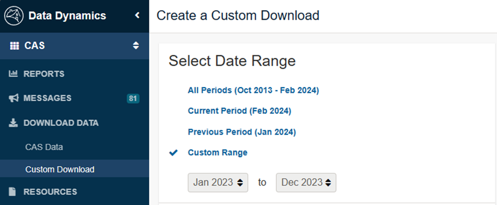
The data used in this example comes from Fannie Mae. It will use the historical loan performance data available through Fannie Mae’s Data Dynamics web portal. This will require you to create an account with Fannie Mae. Once you’ve created an account and logged in, you should see

Steps to Download Data

Data Dynamics

1. Go to Fannie Mae - Data Dynamics - Create a Custom CAS Download
2. Select a deal that is at least 6 months old, a deal with 1-2 years of history will be large enough but not too large
3. Select Data Type - select only Remittance Data
4. Click Generate Files to download a zip file with the performance history

Column Headers

We’ll need a description of the columns to understand what we are loading: Single-Family Loan Performance Dataset and Credit Risk Transfer - Glossary and File Layout. This data isn’t very usable in its current form, so we will use Excel to extract the data from PDF. To extract the data from Excel follow these steps:

1. Download the header PDF file
2. Open up a new, empty worksheet in Excel
3. Go to the Data tab
4. Find the Get Data button on the left of the ribbon
5. Navigate the Get Data menu to go to From File -> From PDF
6. Choose the PDF file to import from
7. Several options will be available on how to import the data, choose the one that works best for you
8. Double check that all columns from the file have been imported to Excel as some may have been cut off

Now, we can use this information to help import our data into BigQuery. This will be used later on.

Uploading Data to Google Cloud Storage

The data we’ve retrieved from Fannie Mae needs to be sent to Google Cloud Storage (GCS). Once the

1. Extract the zip file downloaded from Data Dynamics
2. Navigate to that folder in your console
3. Run the following command to upload all files:

    gsutil cp * gs://{your_bucket_name}/{cas_deal_name}
   

4. Now verify you can see your files in the GCP Console

Creating a BigQuery Table from CSVs

The next step is to create a single table for the multiple CSV files we just uploaded. The difficult part is that we will need to specify a schema for the table. We have to make sure the schema fits the data perfectly as there are no column headers in the CSV files.

The following SQL can be run in the BigQuery Console to load a single table from all the csv files.

LOAD DATA OVERWRITE {dataset_name}.{security_name}
(reference_pool_id STRING,
loan_identifier STRING,
...
)
FROM FILES (
  format = 'CSV',
  field_delimiter = '|',
  uris = ['gs://{your-bucket}/{folder}/*.csv']);

To find an example with all the columns, checkout this sql script.

Now our table has been created, query it to explore the data.

select * from {dataset_name}.{security_name} limit 100;

DBT

DBT (Data Build Tool) is a powerful addition in the modern data stack, enabling analytics engineers to convert raw data in their warehouses into reliable, actionable information. It harnesses the familiar language of SQL, allowing users to define, test, and document their data transformations in a version-controlled environment, promoting collaboration and ensuring data accuracy. With DBT, teams can concentrate more on extracting insights and less on managing data pipelines, speeding up the journey to data-driven decision making.

Installation

1. Setup dbt environment: Assuming python has been setup locally, create a virtual env

   virtualenv dbt-project-env
   source dbt-project-env/bin/activate
   

2. Install bigquery adapter for dbt, this will also install dbt-core

   pip install dbt-bigquery
   

3. Initialize the dbt project and set dbt_dv_data as the project name and select 1 to choose the postgres adapter

   dbt init
   

4. Follow the prompts to configure DBT. This will setup your profiles.yml which the dbt_project.yml will reference. Most importantly this keeps our connection details from being checked into GitHub.
5. Move files from newly created folder. Unfortunately DBT creates everything in a subfolder which isn’t usefull since its easier having it at the same level as the

   mv {dbt_project_folder_created}/* .
   rmdir {dbt_project_folder_created}
   

6. Test with dbt debug

   dbt debug
   

   If your connection to BigQuery is setup properly, you should see All checks passed!.

Cleanup DBT Starter Project

DBT Init gives us some start files. Simply remove the files we don’t need and keep the directory structure.

rm models/example/my_first_dbt_model.sql && 
rm models/example/my_second_dbt_model.sql &&
> models/example/schema.yml

Defining Our First Source

We will use the table we created before as our source. A source is used to define an existing object in the data warehouse that will be referenced by our model. At its simplest, we only need to define where the source is. For BigQuery, we will set the dataset (name) and table name for the source. The GCP Project will be set in our profile and is not specified in this example.

1. Create a directory for our models: models/cas
2. Add file cas_sources.yml
3. Add our source, the table created from the CAS csvs downloaded earlier

sources:
  - name: cas_loanperf # This bigquery dataset the source is in
    tables:
      - name: cas_2022_r01_g1

Add Our First Model

Our first model will reference the source table defined in our yaml file. It will simply read from this table and parse the monthly_reporting_periodcolumn.

1. Create a new file in the models/cas/{cas_deal_name}_clean.sql
2. Add the SQL below:

{{ config(materialized = 'view')}}
WITH with_period AS (
    SELECT
        PARSE_DATE('%m%Y', monthly_reporting_period) AS reporting_period
        ,CAST(current_loan_delinquency_status AS INT64) as current_loan_delinquency_status
        ,* EXCEPT(current_loan_delinquency_status)
    FROM
        {{ source('cas_loanperf', 'cas_2022_r01_g1')}}
)
SELECT
    reporting_period
    ,current_actual_upb + unscheduled_principal_current AS scheduled_ending_balance
    ,SUM(unscheduled_principal_current) OVER (PARTITION BY loan_identifier ORDER BY reporting_period
        ROWS BETWEEN UNBOUNDED PRECEDING AND CURRENT ROW
    ) AS unscheduled_principal_cumulative
    ,SUM(scheduled_principal_current) OVER (PARTITION BY loan_identifier ORDER BY reporting_period
        ROWS BETWEEN UNBOUNDED PRECEDING AND CURRENT ROW
    ) AS scheduled_principal_cumulative
    ,SUM(total_principal_current) OVER (PARTITION BY loan_identifier ORDER BY reporting_period
        ROWS BETWEEN UNBOUNDED PRECEDING AND CURRENT ROW
    ) AS total_principal_cumulative
    ,IF(current_loan_delinquency_status >= 2, 1, 0) as dq60plus
    ,IF(current_loan_delinquency_status >= 3, 1, 0) as dq90plus
    ,IF(current_loan_delinquency_status >= 4, 1, 0) as dq120plus
    ,* EXCEPT (reporting_period)
FROM
    with_period

Compile and Run the Model

Now that we have a source and a model we have enough to run our dbt model.

DBT Compile

First we can run dbt compile to generate executable SQL from our model.

dbt compile will create the defined tables, views, and other objects in our data warehouse

DBT Run

After we’ve viewed our compiled SQL and are happy, we can run dbt run to update the definitions in our data warehouse.

dbt run will create the defined tables, views, and other objects in our data warehouse

Materialization

It is important to pick the proper DBT Materializations for our model.

Materializations are strategies for persisting dbt models in a warehouse. There are five types of materializations built into dbt.

There are 5 types of materializations available in dbt:

• table
• view
• incremental
• ephemeral
• materialized view

The main two materializations you will use are table and view. The first DBT model above uses the view materialization. This means no data is written when the dbt pipeline is run, only the view is created or updated. This is fine, but every time someone calls this view it will read all the data from the underlying table. If this query takes a long time and uses too many resources, a table materialization may be appropriate. In this case the output of the SQL defined in our dbt model will saved to a table.

For our second dbt model, the table materialization will be used. This table aggregates the first table and will only have a few records. So now when we run the dbt model, it will write data to this table.

{{ config(materialized = 'table')}}
SELECT
  reporting_period,
  SUM(unscheduled_principal_current) / SUM(scheduled_ending_balance) AS smm,
  (1 - POW(
    (1 - (SUM(unscheduled_principal_current) / SUM(scheduled_ending_balance)))
    ,12
  )) * 100 as cpr,
  SUM(scheduled_ending_balance) as scheduled_ending_balance,
  SUM(unscheduled_principal_cumulative) as unscheduled_principal_cumulative,
  SUM(scheduled_principal_cumulative) as scheduled_principal_cumulative,
  SUM(total_principal_cumulative) as total_principal_cumulative,
  countif(scheduled_ending_balance > 0) as active_loan_count,
  count(*) as total_loan_count,
  sum(dq60plus) as dq60plus,
  sum(dq90plus) as dq90plus,
  sum(dq120plus) as dq120plus
FROM
    {{ ref("cas_2022_r01_g1_clean")}}
GROUP BY
  reporting_period

Wrapping Up

This small example only touches the surface of some of the great features of DBT. DBT will make managing your data warehouse much easier. Tools such as the lineage view will make maintaining larger project easier. Most importantly, by keeping the entire workflow in SQL we offload the hard work to the data warehouse. This ensures our pipeline can grow as our requirements do.

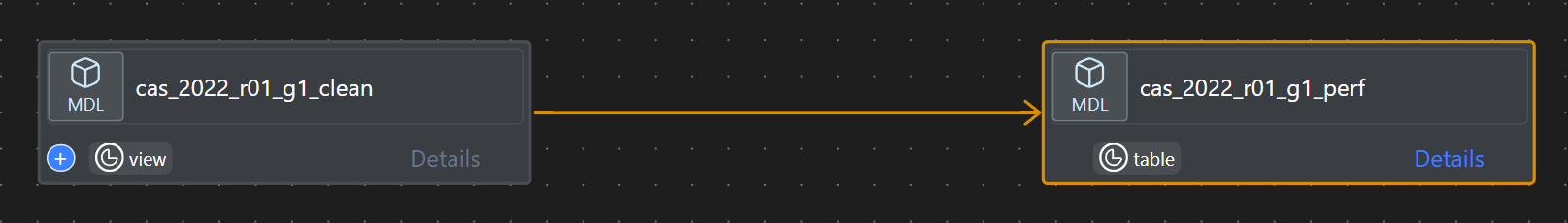DBT Lineage

Display the Results in Plotly Dash

What is the point of all this hard work if we can’t show it off? A quick and easy way to show some performance charts is with Plotly Dash. Here is an example built with Plotly Dash and hosted in GCP Cloud Run. Hopefully, they’ll be time for a post about it soon 🤞.

Plotly Dash Hosted in Cloud Run

Source Code - Plotly Dash

Code for the Plotly Dashboard can be found on GitHub: Loan Performance Dash